A Monte Carlo Study of Argon¶

In short – Using Monte Carlo simulations, the equation of state (EoS) for a 3D fluid of argon is simulated across a wide range of densities.

The fluid made of argon atoms and simulated using monte carlo and python

In 1957, four years after the initial implementation of a Monte Carlo simulation by Metropolis et al. [8, 9], Wood and Parker successfully implemented a 3D Monte Carlo simulation of a fluid using a full Lennard-Jones potential [1]. In their study, Wood and Parker used a Monte Carlo algorithm to predict the Equation of State (EoS) of neutral particles whose parameters were chosen to match those of argon gas. Their results showed good agreement with experimental measurements by Michels on argon [10]. Here, we take advantage of our code to reproduce the results of Wood and Parker for varying density. To follow this project, only Monte Carlo moves are needed. All the chapters up to the Pressure Measurement chapter must have been completed.

Prepare the Python file¶

In a Python script, let us start by importing the constants module of SciPy, and the UnitRegistry of Pint.

from scipy import constants as cst
from pint import UnitRegistry
ureg = UnitRegistry()
ureg = UnitRegistry(autoconvert_offset_to_baseunit = True)

Let up also import NumPy, sys, as well as multiprocessing to launch multiple simulations in parallel:

import sys
import multiprocessing --
import numpy as np

Provide the full path to the code. If the code was written in the same folder as the current Python script, then simply write:

path_to_code = "./"
sys.path.append(path_to_code)

Then, let us import the MinimizeEnergy and MonteCarlo classes:

from MinimizeEnergy import MinimizeEnergy
from MonteCarlo import MonteCarlo

Let us take advantage of the constants module to define a few units, and assign the right units to these variables using the UnitRegistry:

kB = cst.Boltzmann*ureg.J/ureg.kelvin # boltzman constant
Na = cst.Avogadro/ureg.mole # avogadro
R = kB*Na # gas constant

Matching the Parameters by Wood and Parker¶

The interaction parameters must be taken exactly as those from the original publication by Wood and Parker [1]. Wood and Parker provide the value for the position of the energy minimum, \(r^* = 3.822~\text{Å}\), which can be related to \(\sigma\) as:

\[\sigma = r^* \times 2^{-1/6} = 3.405~\text{Å}\]

Wood and Parker also specify the interaction energy for the Lennard-Jones potential, \(\epsilon / k_\text{B} = 119.76\,\text{K}\), from which one can calculate \(\epsilon = 0.238~\text{kcal/mol}\) using the Boltzmann constant \(k_\text{B} = 1.987 \times 10^{-3}\,\text{kcal/(mol·K)}\). From the reduced temperature, \(k_\text{B} T/ \epsilon = 2.74\), one can calculate the temperature \(T = 328.15~\text{K}\) (or \(T = 55~^\circ\text{C}\)).

Within the Python script, write:

epsilon = (119.76*ureg.kelvin*kB*Na).to(ureg.kcal/ureg.mol)
r_star = 3.822*ureg.angstrom
sigma = r_star / 2**(1/6)
m_argon = 39.948*ureg.gram/ureg.mol
T = (55 * ureg.degC).to(ureg.degK)

Here, the mass of argon atoms is used. Note that the mass parameter does not matter for Monte Carlo simulations. Since an average modern laptop is much faster than Wood and Parker’s IBM 701 calculators, let us use a number of particles that is larger than their own numbers of 32 or 108 particles:

N_atom = 200

If you are curious, here is the wikipedia page of the IBM 701.

There are also some parameters that are not explicited by Wood and Parker that we have to choose freely, such as the maximum displacement for the Monte Carlo move, and the cut-off for the Lennard-Jones interaction:

cut_off = sigma*2.5 # angstrom
displace_mc = sigma/5 # angstrom

The choice of \(d_\text{mc}\) does not impact the result, but only impacts the efficiency of the simulation. If \(d_\text{mc}\) is too large, most move will be rejected. If \(d_\text{mc}\) is too small, it will take a very large number of steps for the particles to explore the space. On the other hand, the choice of cutoff may impact the result. The choice of \(r_c = 2.5 \sigma\) is relatively standard and should do the job.

Set the Simulation Density¶

To cover the same density range as Wood and Parker, we will vary the volume of the box, \(V\), so that \(V/V^* \in [0.75, 7.6]\), where \(V^* = 2^{-1/2} N_\text{A} r^{*3} = 23.77 \, \text{cm}^3/\text{mol}\) is the molar volume.

In the Python script, add the following:

volume_star = r_star**3 * Na * 2**(-0.5)
volume = N_atom*volume_star*tau/Na
L = volume**(1/3)

The tau parameter (\(\tau = V/V^*\)) will be used as the control parameter.

Equation of State¶

The Equation of State (EoS) is a fundamental relationship in thermodynamics and statistical mechanics that describes how the state variables of a system, such as pressure \(p\), volume \(V\), and temperature \(T\), are interrelated. Here, let us extract the pressure of the fluid for different density values.

To easily launch multiple simulations in parallel, let us create a function called launch_MC_code that will be used to call our Monte Carlo script with a chosen value of \(\tau = v / v^*\).

Create a new function so that the current script resembles the following:

def launch_MC_code(tau):

    epsilon = (119.76*ureg.kelvin*kB*Na).to(ureg.kcal/ureg.mol)
    r_star = 3.822*ureg.angstrom
    sigma = r_star / 2**(1/6)
    m_argon = 39.948*ureg.gram/ureg.mol
    T = (55 * ureg.degC).to(ureg.degK)

    N_atom = 200

    cut_off = sigma*2.5 # angstrom
    displace_mc = sigma/5 # angstrom

    volume_star = r_star**3 * Na * 2**(-0.5)
    volume = N_atom*volume_star*tau/Na
    L = volume**(1/3)

    folder = "outputs_tau"+str(tau)+"/"

A folder name that will be different for every value of \(\tau\) was also added.

Then, let us call the MinimizeEnergy class to create and pre-equilibrate the system. The use of MinimizeEnergy will help us avoid starting the Monte Carlo simulation with too much overlap between the atoms:

def launch_MC_code(tau):
    (...)
    folder = "outputs_tau"+str(tau)+"/"

    em = MinimizeEnergy(
        ureg = ureg,
        maximum_steps=100,
        thermo_period=10,
        dumping_period=10,
        number_atoms=[N_atom],
        epsilon=[epsilon],
        sigma=[sigma],
        atom_mass=[m_argon],
        box_dimensions=[L, L, L],
        cut_off=cut_off,
        data_folder=folder,
        thermo_outputs="Epot-MaxF",
        neighbor=20,
    )
    em.run()

Then, let us start the Monte Carlo simulation. For the initial positions of the atoms, let us use the last positions from the em run, i.e. initial_positions = em.atoms_positions*em.reference_distance:

def launch_MC_code(tau):
    (...)
    em.run()

    minimized_positions = em.atoms_positions*em.ref_length

def launch_MC_code(tau):
    (...)
    minimized_positions = em.atoms_positions*em.ref_length

    mc = MonteCarlo(
        ureg = ureg,
        maximum_steps=20000,
        dumping_period=1000,
        thermo_period=1000,
        neighbor=50,
        displace_mc = displace_mc,
        desired_temperature = T,
        number_atoms=[N_atom],
        epsilon=[epsilon],
        sigma=[sigma],
        atom_mass=[m_argon],
        box_dimensions=[L, L, L],
        initial_positions = minimized_positions,
        cut_off=cut_off,
        data_folder=folder,
        thermo_outputs="Epot-press",
    )
    mc.run()

Finally, it is possible to call the launch_MC_code function using multiprocessing, and perform the simulation for multiple values of \(\tau\) at the same time (if your computer has enough CPU core, if not, perform these calculations in serial):

if __name__ == "__main__":
    tau_values = np.round(np.logspace(-0.126, 0.882, 10),2)
    pool = multiprocessing.Pool()
    squared_numbers = pool.map(launch_MC_code, tau_values)
    pool.close()
    pool.join()

Here, the 10 requested values of \(\tau\) are 0.75, 0.97, 1.25, 1.62, 2.1, 2.72, 3.52, 4.55, 5.89, and 7.62. Run the script using Python.

When the simulation is done, extract the values of Epot.dat within each folder named outputs_tau0.75/, where 0.75 is the corresponding value of \(\tau\). Disregard the first values of Epot, and only keep the last part of the Monte Carlo simulation. Then, plot p V / RT as a function of V/V^. The results are in good agreement with those of Ref. [1]:

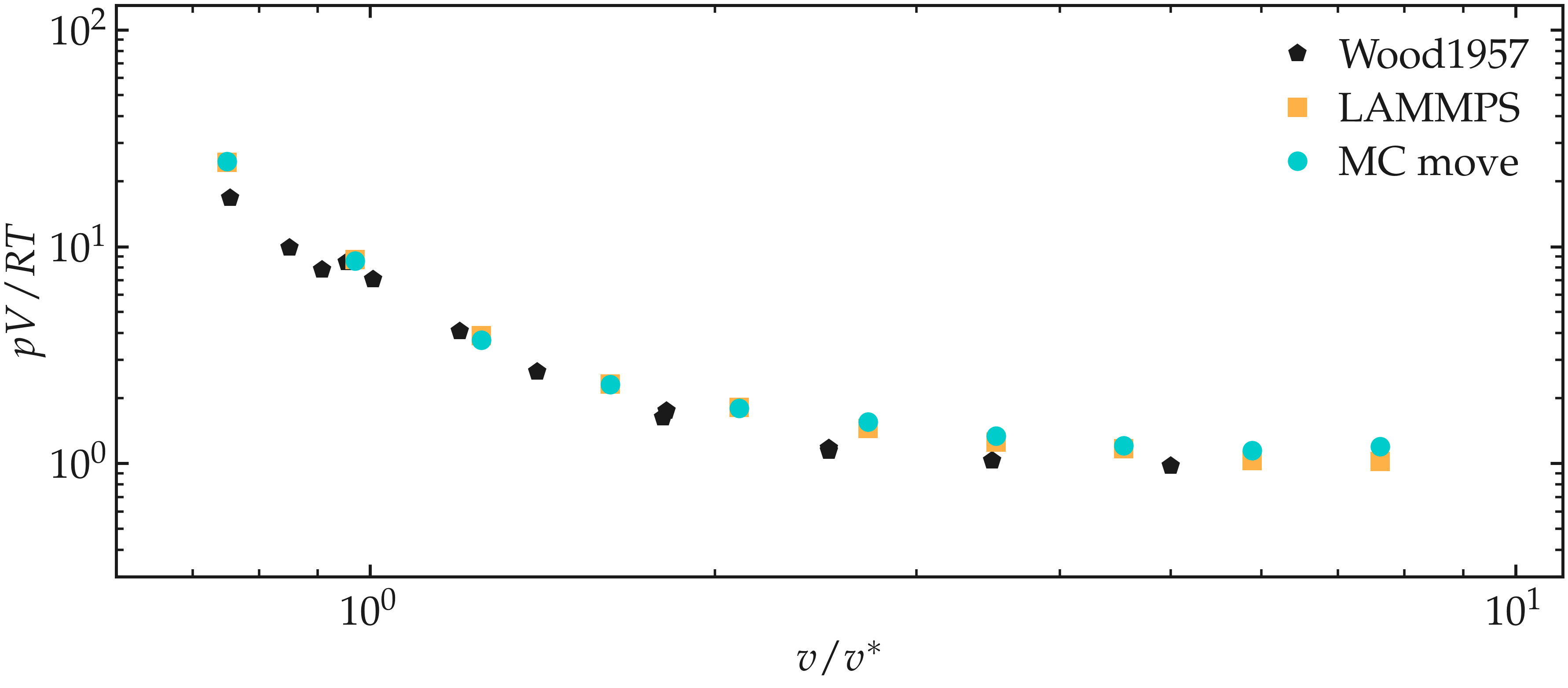
Equation of state of argon as calculated using monte carlo simulation

Figure: Equation of state of the argon fluid as calculated using the Monte Carlo code (disks), and compared with the results from Ref. [1]. Normalized pressure, \(p V / RT\) as a function of the normalized volume, \(V / V^*\), where \(V^*\) is the molar volume. For benchmark purposes, the data obtained using LAMMPS were also added.